How Meta animates AI-generated images at scale
We launched Meta AI with the goal of giving people new ways to be more productive and unlock their creativity with generative AI (GenAI). But GenAI also comes with challenges of scale. As we deploy new GenAI technologies at Meta, we also focus on delivering these services to people as quickly and efficiently as possible.
Meta AI’s animate feature, which lets people generate a short animation of a generated image, carried unique challenges in this regard. To deploy and run at scale, our model to generate image animations had to be able to serve billions of people who use our products and services, do so quickly – with fast generation times and minimal errors, and remain resource efficient.
Here’s how we were able to deploy Meta AI’s animate feature using a combination of latency optimizations, traffic management, and other novel techniques.
Optimizing latency for generating image animations
Before launching the animate feature across our family of apps and on the Meta AI website, making animation models fast was one of our top priorities. We wanted people to see the magic of requesting an animation and seeing it appear in just a few seconds. Not only was this important from a user perspective, but the faster and more efficient we made our model, the more we could do with fewer GPUs, helping us scale in a sustainable way. Our work in creating animated stickers with video diffusion, accelerating image generation with Imagine Flash, and accelerating diffusion models through block caching all helped us develop novel techniques we used to accomplish large latency wins.
Halving floating-point precision
The first of those optimization techniques involved halving floating-point precision. We converted the model from float32 to float16, which speeds up the inference time for two reasons. First, the memory footprint of the model is halved. Second, 16 floating-point operations can be executed faster than 32. For all models, to capture these benefits we use bfloat16, a float16 variant with a smaller mantissa for training and inference.
Improving temporal-attention expansion
The second optimization improved temporal-attention expansion. Temporal-attention layers, which are attending between the time axis and text conditioning, require the context tensors to be replicated to match the time dimension, or the number of frames. Previously, this would be done before passing to cross-attention layers. However, this results in less-than-optimal performance gains. The optimized implementation we went with reduces compute and memory by taking advantage of the fact that the repeated tensors are identical, allowing for expansion to occur after passing through the cross-attention’s linear projection layers.
Leveraging DPM-Solver to reduce sampling steps
The third optimization utilized DPM-Solver. Diffusion probabilistic models (DPMs) are powerful and influential models that can produce extremely high-quality generations—but they can be slow. Other possible solutions, such as denoising diffusion-implicit models or denoising diffusion-probabilistic models, can provide quality generation but at the computational cost of more sampling steps. We leveraged DPM-Solver and a linear-in-log signal-to-noise time to reduce the number of sampling steps to 15.
Combining guidance and step distillation
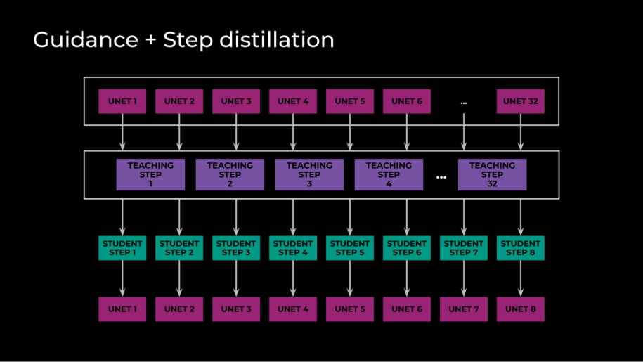
The fourth optimization we implemented combined guidance and step distillation. We accomplished step distillation by initializing a teacher and student with the same weights, and then trained the student to match multiple teacher steps in a single step. Guidance distillation, in contrast, refers to how diffusion models leverage a classifier-free guidance for conditional image generation. This requires both a conditional and unconditional forward pass for every solver step.
In our case, however, we had three forward passes per step: an unconditional, an image-conditional, and a full-conditional, text-and-image step. Guidance distillation reduced these three forward passes into one, cutting inference by a factor of three. The real magic here, though, was combining these two optimizations. By training a student to imitate the classifier-free guidance and multiple steps at the same time with one forward pass through the U-Net, our final model required only eight solver steps, with just one forward pass through the U-Net per step. In the end, during training we distilled 32 teacher steps into eight student steps.

PyTorch optimizations
The final optimization relates to deployment and architecture and involves two transformations. The first was leveraging torch scripting and freezing. By converting the model to TorchScript, we achieved many automatic optimizations. These included continuous folding, fusing multiple operations, and reducing the complexity of the computational graph. Those three optimizations helped to increase inference speed, while freezing allowed further optimization by transforming dynamically computed values in the graph to constants, reducing the total number of operations.
While these optimizations were critical for our initial launch, we have continued to push the boundaries. For example, we have since migrated all of our media inference from TorchScript to use a PyTorch 2.0-based solution, and this resulted in multiple wins for us. We were able to optimize model components at a more granular level with pytorch.compile at the component level, as well as enable advanced optimization techniques such as context parallel and sequence parallel in the new architecture. This led to additional wins, from reducing the development time of advanced features to improvements in tracing and to being able to support multi-GPU inference.
Deploying and running image animation at scale
Once we had fully optimized the model, we had a new set of challenges to tackle. How could we run this model at scale to support traffic from around the world, all while maintaining fast generation time with minimal failures and ensuring that GPUs are available for all other important use cases around the company?
We started by looking at the data for previous traffic on our AI-generated media both at their launches and over time. We used this info to calculate rough estimates of the quantity of requests we could expect, and then used our benchmarking of model speed to determine how many GPUs would be needed to accommodate that quantity. Once we’d scaled that up, we began running load tests to see if we could handle a range of traffic levels, addressing the various bottlenecks until we were able to handle the traffic projected for launch.
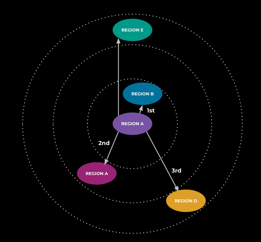
During this testing, we noticed that the end-to-end latency of an animation request was higher than expected—as well as higher than what we had seen after building in all the optimizations described above. Our investigations yielded that traffic was being routed globally, resulting in significant network and communication overhead and adding seconds to the end-to-end generation time. To address this, we utilized a traffic management system that fetches the service’s traffic or load data and uses that to calculate a routing table. The primary objective of the routing table is to keep as many requests as possible in the same region as their requester to avoid having traffic across regions like we were seeing before. The routing table also leverages our predefined load thresholds and routing rings to prevent overload by offloading traffic to other regions when nearing maximum capacity in a region. With these changes, the preponderance of requests remained in region and latency dropped to roughly what we would expect.
Quite a lot of moving parts make this service work. First, it takes each of the metrics that we define for a tier, fetches the value of each from the tier’s machines, and aggregates it by region. It then collects the number of requests per second that each region sends to every other region and uses that to calculate the request-per-second load cost. This tells the system that, generally speaking, the load will increase by X for every added request per second. Once this is complete, the algorithm begins, first by bringing all the traffic to the source region. We don’t yet check if the region has enough capacity or not.
The next step is to enter a loop where during every iteration we look at which region is running closest to maximum capacity. The service tries to take a chunk of that region’s requests and offload them to a nearby region that can handle them without becoming more overloaded. Various levels of overload determine how far away we consider when looking at nearby regions. For example, if the main region is only just starting to run hot, only the closest regions might be utilized. If the region is running at almost maximum capacity, farther-away regions may be unlocked for offloading. We’ll exit the loop if there are no more requests that can be moved between regions, which occurs either when every region is below the defined “overload” threshold or there are no more nearby regions the service can offload to because all nearby regions are also above the threshold. At this point, the service will calculate the optimal number of requests per second for each region and use that to create the routing table mentioned above so our service can appropriately determine where to send traffic at request time.

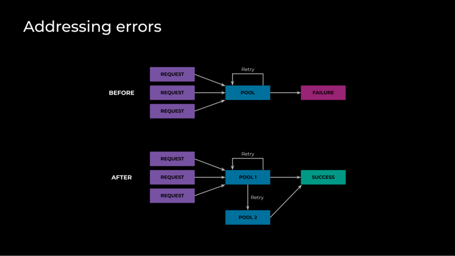
With these optimizations in place, latency returned to levels that we were happy with, but we were seeing a dip in success rate. At a high level, each GPU can only actively work on one request at a time, as each request fully saturates the GPU. To maintain fast latency, it’s imperative that we don’t allow requests to queue up—otherwise, they’ll have a long wait time. To enforce this we made sure that the server load—queued requests plus in-flight requests—is at most one, and that the server rejects other new requests. Because of this, however, when we are running near our capacity limit, we will run into a number of failures. The naive solution to this issue would be to use a queue, but due to having to load balance globally, that presents its own sets of complex challenges to being efficient and fast. What we used instead was approximating by abusing retries to create a probing system that checks for free GPUs really fast and prevents failures.
This worked well before we implemented the traffic management system. That system, while effective at reducing latency, introduced more complications by reducing the number of available hosts for a request, since we no longer had the global routing. We noticed that the retry polling was no longer being helpful and actually tended to cascade if there were any spikes. Further investigation led us to discover that our router needed to have more optimized settings for retries. It had neither delay nor backoff. So if we had a region where lots of tasks were trying to run, it was stuck overloading until it started failing requests. To avoid the cascading errors, we modified these retry settings to add a marginal execution delay to a percentage of jobs at scheduling time—making them available to execute gradually instead of all at once—as well as an exponential backoff.
Once all of this was done, we had a deployed model that was highly efficient, functioned at scale, and could handle global traffic with high availability and a minimum failure rate.

Read more
To learn more about our work developing and deploying GenAI to animate images, read:
Animated Stickers: Bringing Stickers to Life with Video Diffusion
Imagine Flash: Accelerating Emu Diffusion Models with Backward Distillation
Cache Me if You Can: Accelerating Diffusion Models through Block Caching
The post How Meta animates AI-generated images at scale appeared first on Engineering at Meta.
目录
最新
- ILA Evo: Meta’s journey to reimagine fiber optic in-line amplifier sites
- Indexing code at scale with Glean
- Translating Java to Kotlin at Scale
- How we think about Threads’ iOS performance
- How to build a mixed reality headset
- Inside Facebook’s video delivery system
- Typed Python in 2024: Well adopted, yet usability challenges persist
- Powering AI innovation by acccelerating the next wave of nuclear